

Linear Regression

Graduated in 2021. Later worked as an Associate for 6-months in MNC. Later joined the fellowship at BootCamp in backend development. Currently preparing for interviews.
Introduction
Hey there, fellow data enthusiasts! Today, we're going to dive deep into one of the most straightforward yet powerful algorithms in Machine Learning: Linear Regression.
Have you ever wondered how businesses predict sales for the upcoming month? Or how economists forecast unemployment rates? Well, a lot of that magic can be attributed to Linear Regression. Buckle up, and let's break this down!
Math Behind
At its core, linear regression revolves around finding the best linear relationship (or a straight line) that can predict our target variable based on one or more predictors. Mathematically, this can be represented as:
y=β0+β1x1+β2x2+...+βnxn+ϵ
Here:
y is our dependent variable (the one we want to predict).
x1,x2,...,xn are our independent variables.
β0 is the intercept.
β1,β2,...,βn are coefficients for the independent variables.
ϵ is the error term.
Our main objective is to find values for β0,β1,...,βn such that they minimize the difference between the predicted and actual values of y. This difference is commonly known as the "cost" or "error".
We usually use the Mean Squared Error (MSE) to measure this:
MSE=n1∑i=1n(yi−y^i)2 Where:
yi is the actual value.
y^i is the predicted value.
n is the number of observations.
Graphical Representation
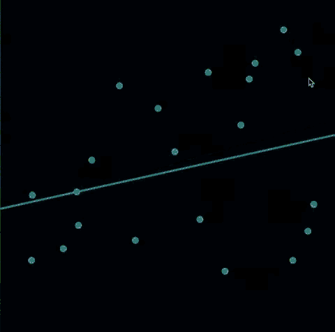
The beauty of linear regression is that it can be visualized easily, especially when dealing with just one independent variable (also known as simple linear regression). The relationship between the dependent and independent variable is represented as a straight line, aptly termed the "regression line."
This line is chosen in such a way that the cumulative difference (or "error") between the actual data points and the points on the regression line is minimal. When you plot the data and the regression line on a graph, you'll notice that some data points lie above the line and some below. The vertical distance between each data point and the line represents the error for that particular point.
import matplotlib.pyplot as plt
import numpy as np

# Sample data and model prediction
X = np.array([1, 2, 3, 4, 5])
y = np.array([2, 4, 5, 4, 5])
y_pred = model.predict(X.reshape(-1, 1))

plt.scatter(X, y, color='blue', label='Actual Data Points')
plt.plot(X, y_pred, color='red', label='Regression Line')
plt.xlabel('X (Independent Variable)')
plt.ylabel('y (Dependent Variable)')
plt.legend()
plt.title('Linear Regression Graphical Representation')
plt.show()
The magic behind finding the best-fit line is in the optimization process, which involves some calculus. The goal is to minimize the Mean Squared Error (MSE) and to do that, we need to find where the MSE is at its lowest point. This is where differentiation comes into play!
Remember our MSE equation:
MSE=n1∑i=1n(yi−y^i)2
To minimize the MSE, we take its derivative concerning the coefficients β and set it to zero. This gives us the gradient descent update equations:
βj:=βj−α∂βj∂(MSE)
Where:
βj is the coefficient being updated.
α is the learning rate, a hyperparameter that determines the step size in the direction of the steepest decrease in MSE.
By iteratively updating the coefficients using the above equation, we move towards the values of β that minimize our cost function, MSE. This iterative method is known as "gradient descent."
Implementation
Now, let's roll up our sleeves and see how we can implement this in Python. I'll be using the sklearn library, which provides an easy-to-use interface for Linear Regression.
# Importing necessary libraries
from sklearn.linear_model import LinearRegression
from sklearn.model_selection import train_test_split
from sklearn.metrics import mean_squared_error

# Sample data
X = [[1], [2], [3], [4], [5]]
y = [2, 4, 5, 4, 5]

# Splitting data into training and testing sets
X_train, X_test, y_train, y_test = train_test_split(X, y, test_size=0.2, random_state=42)

# Creating a linear regression model
model = LinearRegression()

# Training the model
model.fit(X_train, y_train)

# Predicting using the model
y_pred = model.predict(X_test)

# Calculating MSE
mse = mean_squared_error(y_test, y_pred)
print(f"Mean Squared Error: {mse}")
Conclusion
Linear Regression, despite its simplicity, is a mighty tool in the hands of data scientists and statisticians. It provides a foundational understanding of how we can make predictions from our data. As you dive deeper into the world of Machine Learning, you'll come across more sophisticated algorithms, but the core principles you learn from linear regression will always guide you.


